Report builder window
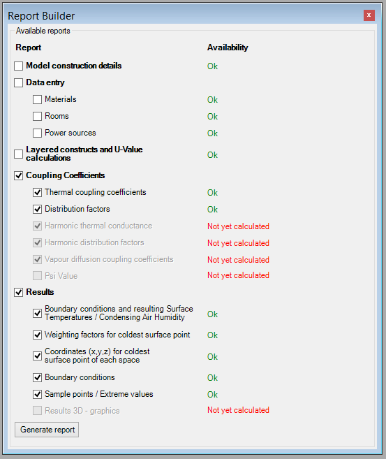
The report builder enables you to create a fully customized report. You can select the parts you need for your report from a variety of predefined report modules.
The report builder consists of a table with 2 columns and a button to initiate report generation. The first column shows the report modules and the second column displays the availability of the module. To select a report module for inclusion into the report to generate, simply check the check box next to it.
The report modules are grouped according to the frequency they are printed together in one report. If you check/uncheck a report module group, all modules will get checked/unchecked.
The availability of a module depends on several factors: A report module may not be available, because the current model doesn't contain the features the report relies on. E.g., if your model doesn't contain power sources, the power sources report won't be available. The availability of some report modules also depends on the state of calculation execution. If you didn't yet execute the thermal coefficients calculation, the respective report won't be available.
Finally, if you've selected all modules according to your needs, you can generate a report by simply clicking on the button at the bottom of the form. This will open the report viewer window.
Report modules
The report modules are grouped into these groups:
- Model construction details
- Data entry
- Layered constructs and U-Value calculations
- Coupling coefficients
- Results
Each of those groups and the entailed modules will be further explained in the subsequent sections.
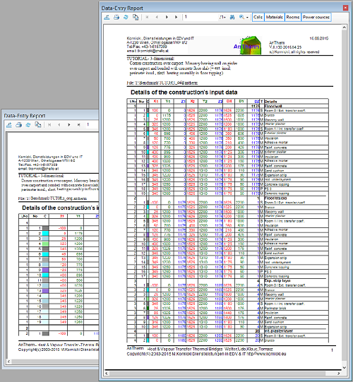
Model construction details report
The model construction details group doesn't have child modules, but is a rather module by itself. This module displays all input elements of the model with the following details:
- Element number
- Color of the element in the model
- Element coordinates (color-coded)
- Element type
- Element details
This is a fairly large report module. It can be printed in presentation or landscape layout.
![]() Remark:
Data of vapour diffusion resistance μ will be also reported if
entered.
Remark:
Data of vapour diffusion resistance μ will be also reported if
entered.
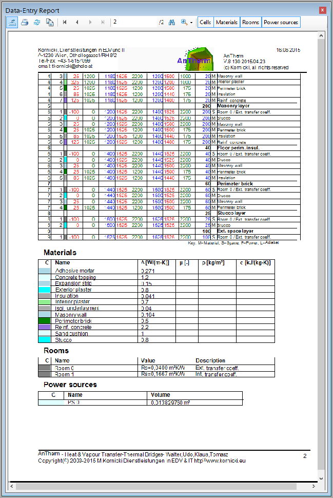
Data entry reports
The data entry report groups contains the modules
- materials,
- rooms and
- power sources.
The report is used for summarizing documentation of all building components data relevant for the simulation.
Compared to the model construction details report only data relevant for the calculation is reported. Resulting from the overlapping elements some materials might have no impact within calculation (being fully overlapped and thus discarded). Thus this report shall be used to document and to verify the input of spaces and power sources (boundary conditions), their names and transfer coefficients.
Remark: If there are power sources included in the model (after all overlapping of elements have been resolved) their resulting (active) volumes will be calculated and output also. This values might be helpful during the entry of boundary conditions.
![]() Remark:
Data of vapour diffusion resistance μ will be also reported if
entered.
Remark:
Data of vapour diffusion resistance μ will be also reported if
entered.
Layered constructs and U-Value calculations report
This report lists U-Values of characteristic
layered constructs at adiabatic boundaries of the model.
These intermediary results are required for the calculation of
thermal bridge
correction factor Psi or Chi.
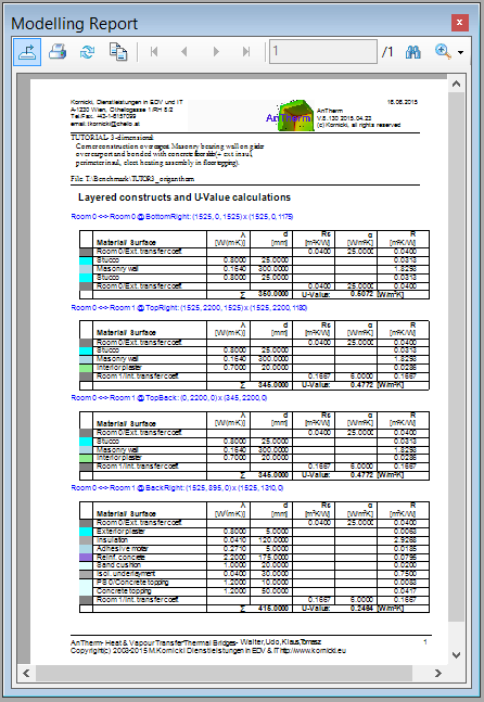
Remark: The listing does only show U-Values of layered
constructs between two spaces; Incomplete layered constructs will not be output.
The algorithm searches at all six sides of the model bounding box for adiabatic
cut-off planes (from outside towards model's interior, the first one adiabatic
plane in each such direction). If a space surface is found at first in one of
that directions, then there will be no adiabatic boundary reported in that
direction. Adiabatic planes found by that process are then intersected in pairs
at twelve edges. At these intersection lines U-Value profiles are generated -
each such profile results in none, one or even many layered constructs
space-to-space.
Remark: For U-Value profiles passing multiple layered constructs (e.g.
multiple ceilings) there will be multiple U-Values reported for respective space
pairs.
For detailed report of all data entered, including the detailed listing of all elements, please use model construction details report.
Coupling coefficients reports
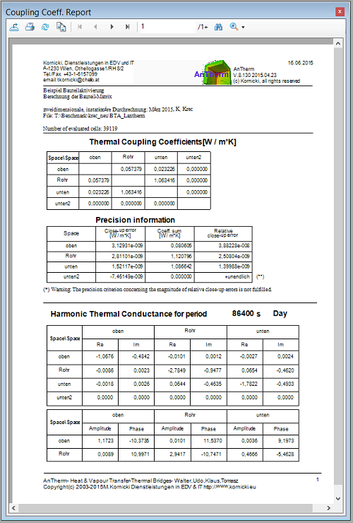
The Coupling Coefficients and Precision report displays the matrix Li,j
of thermal coupling coefficients (L2D or L3D , also called heat transfer coefficients H in
some standards
or Leitwert matrix, thermal conductance matrix) and respective
precision information of the
simulation.
For a two dimensional model the matrix shows length related transmittance L2D [Wm−1K−1]
; for three dimensional construction the matrix displays thermal coupling
coefficients L3D per se [WK−1].
Depending on which problems have been chosen for the Solver and on the number and type of boundary conditions following results are shown:
- Number of evaluated cells (size of the system of equations)
for the steady state (stationary) heat transport problem:
- matrix of stationary, steady state thermal coupling coefficients for all space pairs
- heat distribution factors for all power sources and spaces
- precision information for the steady state heat transfer problem
for the steady state vapour diffusion problem:
- precision information for the steady state vapour diffusion problem
for the dynamic, transient, harmonic, periodic heat transport problem, for any period length (and eventually higher harmonics):
- the matrix of harmonic coupling coefficients for all space pairs,
- the harmonic heat distribution factors of each source to all spaces
given as complex numbers and as amplitude/phase pairs.
If the number of matrix columns output shall overrun the page width then the output of overrunning matrix columns is continued in groups one below the other.
Steady state (stationary) thermal coupling coefficients
The report displays the matrix of thermal coupling coefficients for any pair of spaces (with 6 decimal places).
If N spaces are attached to the considered construction the NxN matrix will be displayed (without diagonal elements).
Theoretically the matrix shall be symmetrical (i.e. Lij=Lji), thus the output allows precision consideration of results.
These values are used, for example, to calculate thermal bridge correction
factors - for a 3D case the "point thermal transmittance" Χ (Chi) and for a 2D
case the "linear thermal transmittance" Ψ (Psi).
See also:
Psi-Value Determination (Calculate Ψ-Value)
Remark: By multiplying the (steady state) thermal coupling coefficient Lij by the difference of temperatures of respective space pairs Θi−Θj one will receive the heat stream (or the length related heat stream in 2D case) between the two spaces transmitted through the modelled component.
Heat source Distribution Factors (steady state)
In the event heat sources are available also, the heat distribution factors of each source to all spaces are shown too.
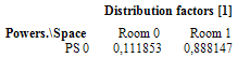
If N spaces are attached to the considered construction then there will be N numbers shown for every heat source in the distribution table. The i-th (i = 1,N) column value of the distribution table shows the percentage of the heat provided by the particular heat source passing to the i-th space. The values of the distribution table are therefore from the range 0 to 1.
Because the steady state calculation does not cover the heat capacity storage, the sum of all distribution values must theoretically result in 1 (apart from minor rounding errors) allowing further precision consideration of results.
Remark: By multiplying the distribution factor Fkj by its respective power density Φk of the heat source k and its volume Vk one will receive the heat stream (or the length related heat stream in 2D case) from the heat source k to the space j. (The volume of every heat source will be shown within Modelling report or Results report).
Transient (instationary, dynamic), harmonic, periodic thermal coupling coefficients
Provided the solution of a dynamic, transient, harmonic, periodic problem has been computed also, the matrix of periodic harmonic coupling coefficients will be output (with output of up to 4 decimal places).
The output is provided for each requested period (period length, in decreasing
order; longest first) once as matrix
of complex numbers and additionally as matrix of norm (amplitude) and argument
(phase shift, time lag) values.
From that output the exterior harmonic coupling coefficient (between exterior
and interior) can be identified for example.
Diagonal elements (contrary to the steady state case these are significant and output here) can be used for the calculation of effective heat capacities.
Theoretically, as for the steady state case, the matrix shall be symmetrical, thus the output allows precision considerations of results also.
In the event heat sources are available also, the harmonic heat distribution factors of each source to all spaces are shown too.
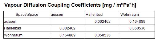
Vapour diffusion, hygric coupling coefficients
![]() The
report will also show hygric coupling coefficients
(mg/Pa*h) ("Matrix of hygric coupling") if there are results of
vapour diffusion calculation available too.
The
report will also show hygric coupling coefficients
(mg/Pa*h) ("Matrix of hygric coupling") if there are results of
vapour diffusion calculation available too.
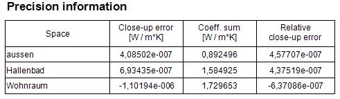
Precision information
An immediate indicator of the precision of the solutions is the matrix of thermal coupling coefficients itself - if it is not reasonably symmetrical, then further calculation might be necessary. Along with the output of coupling coefficients the necessary information about the precision of these results is output.
A theoretically exact method of calculation would necessarily satisfy the condition, that the sum of heat entering a component exactly equals the sum leaving the same - for any set of basic solutions. The inherent nature of a numeric method, however, will always result in a marginal difference in the evaluated energy balance. This is referred to here as the close-up error of base solution. Dividing the close-up error by the sum of the coefficients associated with the respective base solution (space) provides a measure of the precision of calculation.
The relative close-up error shall never exceed 10−4 considering precise solution (see EN ISO 10211:2008).
The value of the Relative Close-Up Error limit (default 10−4) can be adjusted within application settings:
- If the relative close-up error exceeds the half of that limit the line will be marked with (*) - i.e. "just at minimum precision".
- If the relative close-up error exceeds that limit (**) are shown.
A warning message "(*) Warning: The precision criterion concerning the magnitude of relative close-up errors is not fulfilled" will be shown below the precision data listing if the precision criterion is not satisfied by any of base solution (the display of this message can be turned off by the application setting "Relative Close-Up Error - Warn if above").
Note: If the relative close-up error exceeds 10−4 (or the limit otherwise set) a continuation of calculation based on more stringent parameters for more precise solution should be considered before proceeding with further evaluation. Eventually modified (finer or coarser) raster discretisation (gridding) might be required also.
![]() If the
solution of vapour diffusion has been also computed, the associated precision
information is also displayed following the results of thermal heat calculation.
If the
solution of vapour diffusion has been also computed, the associated precision
information is also displayed following the results of thermal heat calculation.
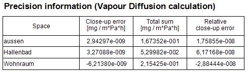
Precision indicators, i.e. (*), (**) and a warning message, are shown for the vapour base solutions - based on same precision criteria (see above).
Results reports
The Results report provides the output related to boundary conditions applied and shows results for coldest surface points of each respective space and includes their temperatures, coordinates and temperature weighting factors also.
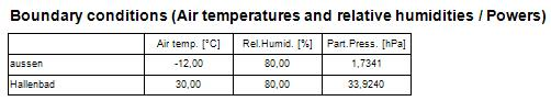
Calculation of evaluation results dependant on boundary conditions is requested by applying these values from the Boundary Conditions window.
The results offered by this report are used for the assessment of fulfilling (or failing) the condensation and mould growth avoidance criteria (see EN ISO 13788).
For each space the application automatically locates points of lowest surface temperature and outputs its coordinates. Also g-values (the weighting factors) are calculated and output.
Along temperatures of coldest surface points the application outputs respective dew point values (maximum non-condensing air humidity) also [1]. Respective values are calculated according to formulas of partial pressure as defined in EN ISO 13788:2002.
The evaluation is executed on top of base solutions solved and superposed with respective boundary conditions (reported by the number of equations or cells solved) then further refined to the super fine solution (reported by the number of nodes evaluated).
Boundary conditions and critical results
For each space connected to the model following results information is offered:
- name of the space
- air temperature (the boundary condition of that space as entered within the Boundary Conditions window and applied)
- the lowest surface temperature θ*Rsi at the surface of that space (at the coldest surface point)
- the highest surface temperature at the surface of that space (at the hottest surface point)
- highest allowed relative air humidity with respect to the coldest surface point of that space to avoid surface condensation (condensing humidity, Condens. RH)
- the temperature factor f*Rsi with respect to the coldest surface point θ*Rsi (see remarks below)
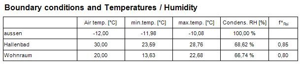
The temperature factor f*Rsi will be evaluated against the space with the lowest temperature Θe (i.e. that space will be assumed to be "exterior") and calculated according to standard by the definition f*Rsi = (θ*Rsi − θe)/(θi − θe) .
Remark: In a two space case temperature factors f*Rsi will be output in addition to temperature weighting factors g - calculated for points of lowest temperatures of surface of each space. The temperature factor f*Rsi can be used as construction characteristic indicator only when two boundary conditions are applied. When three or more boundary conditions (spaces, power sources) are involved then the standard requires using of temperature weighting factors g because f*Rsi is not suitable in such cases!.
Remark: The output of
temperature factors f*Rsi will be suppressed if the
application setting "fRsi - Two-Space only evaluation"
is turned on and there are more than exactly two temperature
boundary conditions involved in the model.
If there are more then exactly two temperature boundary
conditions and the application setting "fRsi - Two-Space only evaluation"
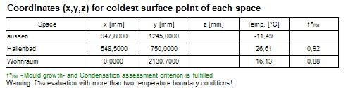
is kept turned off, then the appropriate warning message is displayed within the report: "Warning: fRsi evaluation with more
then two temperature boundary conditions!".
If heat sources are also modelled:
- the overall power of the heat source (calculated from the boundary condition entered and its volume)
- the power density (the boundary condition of that heat source as entered within the Boundary Conditions window and applied)
- the effective volume of that heat source
Remark: The assessment of further extreme values (e.g. temperatures) at all surfaces and within interiors of all power sources is provided within the 2nd part of this report too.
Weighting Factors (g-values) of coldest space points
The weighting factors (g-values) will be output as a matrix for the coldest point of every space. Every column of the matrix displays g-values for the coldest point of the space surface named in the column heading.
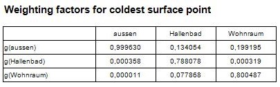
Weighting factors g are characteristic for respective points of the construction and their value is independent from any boundary conditions. The summation of g-values of a point multiplied by the respective boundary condition results in the temperature of that point. Under the assumption that the location of extreme poles will not change under different boundary conditions one can easily calculate the resulting temperature at these varied boundary conditions.
Remark: The sum over all g-values belonging to temperature boundary conditions at specific point (sum of values in one column without those belonging to heat sources) is always 1.
Remark: If the number of matrix columns output shall overrun the page width then the output of overrunning matrix columns is continued in groups one below the other.
Coordinates of coldest surface points
The listing of points of lowest space surface temperatures for each space shows point coordinates, the respective surface temperature, the dew point and the temperature factor f*Rsi also.
Condensation and Mould Growth Assessment Criteria
If requested by the application setting "fRsi,min design factors - Warn if undercut" (on by default) AnTherm will automatically evaluate the assessment of the f*Rsi values by comparing actual values of f*Rsi to their design values for condensation free and mould-growth free constructions (also set within application settings).
- shall the actual value of f*Rsi undercut the design value for mould-growth free construction, the indicator (*) is shown
- shall the actual value of f*Rsi undercut the design value for condensation free construction (and eventually mould-growth criteria too), the indicator (**) is shown
In addition, if either of the design values are undercut at any space surface there will be warning message displayed at the end of this report:
- (*) Warning: f*Rsi < XXXX - Mould growth assessment criterion not fulfilled.
- (**) Warning: f*Rsi < XXXX - Condensation assessment criterion not fulfilled.
If the criteria is fulfilled on the other hand following confirmation will be printed:
- f*Rsi - Mould growth- and Condensation assessment criteria are fulfilled.
Remark: The output of
temperature factors f*Rsi will be suppressed if the
application setting "fRsi - Two-Space only evaluation"
is turned on and there are more than exactly two temperature
boundary conditions involved in the model.
If there are more then exactly two temperature boundary
conditions and the application setting "fRsi - Two-Space only evaluation"
is kept turned off, then the appropriate warning message is displayed within the report: "Warning: fRsi evaluation with more
then two temperature boundary conditions!".
Probe Points report
The Probe Points report us used for the output of temperatures at chosen probe points at currently applied boundary conditions .
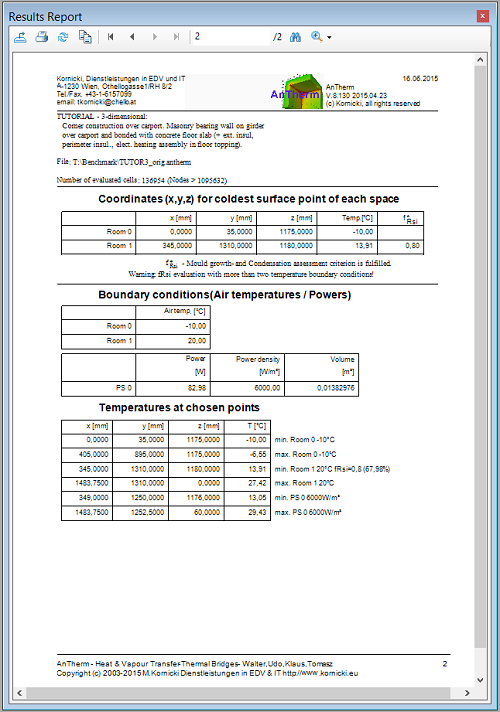
The report outputs temperatures at points (coordinates x,y,z) defined in the window "Probe Points".
For each point given the application outputs coordinates (values of x,y,z) and the value of calculated temperature. If required a tri-linear interpolation is used to calculate temperature exactly at any point of the model from node values available at the super fine grid.
If the chosen point is located at some space surface the respective dew point (maximum non-condensing air humidity) is calculated and output in %.
If the chosen point is located outside of the boundaries of the construction only its coordinates are output.
Remark: The report includes points of lowest and highest surface temperature for each space surface automatically – space name, space temperature, dew point and f*Rsi value (if applicable) are output – same as in Results report.
Remark: The output of temperature factors f*Rsi will be suppressed if the application setting "fRsi - Two-Space only evaluation" is turned on and there are more than exactly two temperature boundary conditions involved in the model.
Remark: If there are power sources contained within the model this report also includes points of lowest and highest temperature within each power source (to assess overheating for example).
If there is solution of vapour diffusion available also, values of saturation and partial pressure are also output at each point:

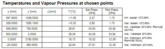
If the current value of partial pressure is higher then saturation pressure, a star (*) is shown adjacent to the partial pressure value - this shall alert on possible condensation risk at this respective point.
| VAPOUR-option: Analysis of multidimensional vapour diffusion is only possible with an active VAPOUR-Option of the program.. |
 |
Remark: Point evaluated are defined in the
window Probe Points. The
list of probe points can be extended directly from
Results 3D window (Probe) also.
Remark: Shall partial solution be only available to the report (e.g. some base solution yet not calculated finally, spaces without thermal connection with the model, etc.) the respective result fields will be left empty. Please consider checking the input data or rerunning the solver and checking the output shown within the solver window in such situation.