Comparing Results under Different Conditions
The same model shall now be evaluated under the condition of an active heat source element. The electric heating assembly embedded in the floor is assumed to have a power output of 60 W/m2. In the two-dimensional simulation, which is modelled as a layer of 1 m thickness, this output corresponds to 60 Watts per meter length of heating element in the section. The power density of such 10 mm thick heating assembly is then:
60 W/m2 / 0.010 m → 6000 W/m 3
and this is what has to be provided as input to the program. This also show how to calculate the power density based on manufacturer data and construction entered.
Alternatively one could calculate the total power of the source and divide it by the resulting volume. The total power to be assigned to the heat source here is therefore:
60 W/m2 x 1.176 m x 1.000 m → 70.56 W
Having that and the total volume of the power source (this can be obtained from earlier basic reports) On the other hand, for the two-dimensional simulation being modelled as a layer of 1 m thickness the power density of the whole heat source results in:
70.56 W / 0.01176
m 3 → 6000 W/m 3 .
or
70.56 W / (1.176 m x 1.000 m x 0.010 m)
→ 70.5 W / 0.01176m 3 = 6000 W/m 3 .
and this is what has to be provided as input to the program and same as the value computed earlier above.
To re-define the conditions of evaluation, activate the window Boundary conditions (if hidden turn to View→Evaluation→Boundary Conditions). Move the cursor to the power input field (the temperature values can be left as they are) and enter the new power density value [W/m3]:
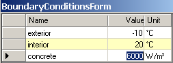
Confirm the entry with Apply.
Numeric Results
Since the conductance matrix and heat source distribution factors remain the same for any given evaluation conditions, these need not be printed out again.
The Evaluation results printout, however, does show new data:
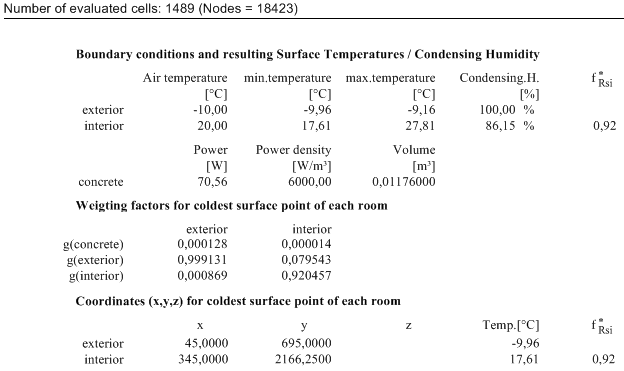
The coldest interior surface point is no longer at the floor/wall corner. The temperature on the floor surface is also considerably warmer than without the heat source (nearly 8° higher).
Graphic Results
Having the graphic results window open from the previous evaluation the significant change could be observed.
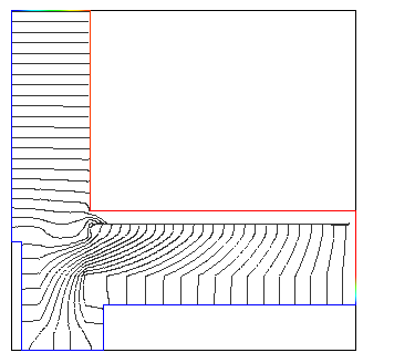
Note different shape of streamlines drawn!
Let's change back to single streamline view (turn all Slices on, select streamline to start at Slice X/Y/Z and eventually change the tube radius back to earlier value of about 12 and colorizing on).
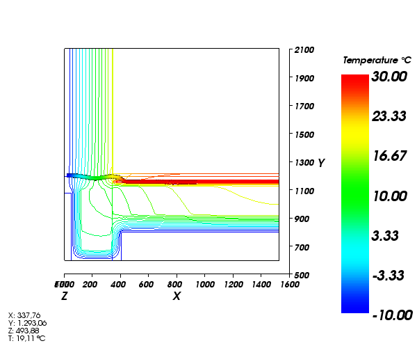
Now turn the isolines back on to see the temperature distribution.
This time the evaluation range of temperatures is noticeably broader. As could be expected, the isotherm lines, drawn at the same temperature interval as before, are highly concentrated in the insulation.
Please go to Isotherms an adjust the evaluation range properly to reflect the change. Also the Colorbar needs some adjustment for this new, extended, range of temperatures to be coloured sufficiently. This is the matter of choice if you want same colour structure be kept for comparative analysis with the earlier (powerless) evaluation or not.
This chapter is not finished yet. More evaluation examples shall be included here later on.
> Continue reading with "Three-dimensional Analysis"...