Coupling Coefficients and Precision report
 The Coupling Coefficients and Precision report displays the matrix Li,j of thermal coupling coefficients (L2D or L3D , also called heat transfer coefficients H in some standards or Leitwert matrix, thermal conductance matrix) and respective precision information of the simulation.
For a two dimensional model the matrix shows length related transmittance L2D [Wm−1K−1] ; for three dimensional construction the matrix displays thermal coupling coefficients L3D per se [WK−1].
Depending on which problems have been chosen for the Solver and on the number and type of boundary conditions following results are shown:
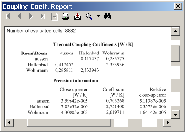
- Number of evaluated cells (size of the system of equations)
for the steady state (stationary) heat transport problem:
- matrix of stationary, steady state thermal coupling coefficients for all space pairs
- heat distribution factors for all power sources and spaces
- precision information for the steady state heat transfer problem
for the steady state vapour diffusion problem:
- precision information for the steady state vapour diffusion problem
for the dynamic, transient, harmonic, periodic heat transport problem, for any period length (and eventually higher harmonics):
- the matrix of harmonic coupling coefficients for all space pairs,
- the harmonic heat distribution factors of each source to all spaces
given as complex numbers and as amplitude/phase pairs.
If the number of matrix columns output shall overrun the page width then the output of overrunning matrix columns is continued in groups one below the other.
Steady state (stationary) thermal coupling coefficients
The report displays the matrix of thermal coupling coefficients for any pair of spaces (with 6 decimal places).
If N spaces are attached to the considered construction the NxN matrix will be displayed (without diagonal elements).
Theoretically the matrix shall be symmetrical (i.e. Lij=Lji), thus the output allows precision consideration of results.
These values are used, for example, to calculate thermal bridge correction factors - for a 3D case the "point thermal transmittance" Χ (Chi) and for a 2D case the "linear thermal transmittance" Ψ (Psi).
See also: Psi-Value Determination (Calculate Ψ-Value)
Remark: By multiplying the (steady state) thermal coupling coefficient Lij by the difference of temperatures of respective space pairs Θi−Θj one will receive the heat stream (or the length related heat stream in 2D case) between the two spaces transmitted through the modelled component.
Heat source Distribution Factors (steady state)
In the event heat sources are available also, the heat distribution factors of each source to all spaces are shown too.
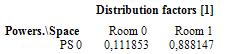
If N spaces are attached to the considered construction then there will be N numbers shown for every heat source in the distribution table. The i-th (i = 1,N) column value of the distribution table shows the percentage of the heat provided by the particular heat source passing to the i-th space. The values of the distribution table are therefore from the range 0 to 1.
Because the steady state calculation does not cover the heat capacity storage, the sum of all distribution values must theoretically result in 1 (apart from minor rounding errors) allowing further precision consideration of results.
Remark: By multiplying the distribution factor Fkj by its respective power density Φk of the heat source k and its volume Vk one will receive the heat stream (or the length related heat stream in 2D case) from the heat source k to the space j. (The volume of every heat source will be shown within Modelling report or Results report).
Transient (instationary, dynamic), harmonic, periodic thermal coupling coefficients
Provided the solution of a dynamic, transient, harmonic, periodic problem has been computed also, the matrix of periodic harmonic coupling coefficients will be output (with output of up to 4 decimal places).
The output is provided for each requested period (period length, in decreasing order; longest first) once as matrix of complex numbers and additionally as matrix of norm (amplitude) and argument (phase shift, time lag) values.
From that output the exterior harmonic coupling coefficient (between exterior and interior) can be identified for example.
Diagonal elements (contrary to the steady state case these are significant and output here) can be used for the calculation of effective heat capacities.
Theoretically, as for the steady state case, the matrix shall be symmetrical, thus the output allows precision considerations of results also.
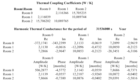
In the event heat sources are available also, the harmonic heat distribution factors of each source to all spaces are shown too.
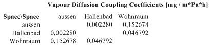
Vapour diffusion, hygric coupling coefficients
![]() The report will also show hygric coupling coefficients (mg/Pa*h) ("Matrix of hygric coupling") if there are results of vapour diffusion calculation available too.
The report will also show hygric coupling coefficients (mg/Pa*h) ("Matrix of hygric coupling") if there are results of vapour diffusion calculation available too.
Precision information
An immediate indicator of the precision of the solutions is the matrix of thermal coupling coefficients itself - if it is not reasonably symmetrical, then further calculation might be necessary. Along with the output of coupling coefficients the necessary information about the precision of these results is output.
A theoretically exact method of calculation would necessarily satisfy the condition, that the sum of heat entering a component exactly equals the sum leaving the same - for any set of basic solutions. The inherent nature of a numeric method, however, will always result in a marginal difference in the evaluated energy balance. This is referred to here as the close-up error of base solution. Dividing the close-up error by the sum of the coefficients associated with the respective base solution (space) provides a measure of the precision of calculation.
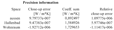
The relative close-up error shall never exceed 10−4 considering precise solution (see EN ISO 10211:2008).
The value of the Relative Close-Up Error limit (default 10−4) can be adjusted within application settings:
- If the relative close-up error exceeds the half of that limit the line will be marked with (*) - i.e. "just at minimum precision".
- If the relative close-up error exceeds that limit (**) are shown.
A warning message "(*) Warning: The precision criterion concerning the magnitude of relative close-up errors is not fulfilled" will be shown below the precision data listing if the precision criterion is not satisfied by any of base solution (the display of this message can be turned off by the application setting "Relative Close-Up Error - Warn if above").
Note: If the relative close-up error exceeds 10−4 (or the limit otherwise set) a continuation of calculation based on more stringent parameters for more precise solution should be considered before proceeding with further evaluation. Eventually modified (finer or coarser) raster discretisation (gridding) might be required also.
![]() If the solution of vapour diffusion has been also computed, the associated precision information is also displayed following the results of thermal heat calculation.
If the solution of vapour diffusion has been also computed, the associated precision information is also displayed following the results of thermal heat calculation.
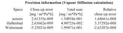
Precision indicators, i.e. (*), (**) and a warning message, are shown for the vapour base solutions - based on same precision criteria (see above).
A report can be:
- viewed on the screen
- saved as PDF, XLS, DOC or RTF file
- printed onto a printer
- searched by keywords
See Toolbar of a Report window
See also: Evaluation windows, Evaluation and Results, Toolbar of a Report window, Results 3D window, Boundary Conditions window, Please Wait window, Psi-Value Determination (Calculate Ψ-Value), Linear and Point Transmittance, EN ISO 10211